In this article I will talk about how to find the average standard deviation . This material is extremely important for a full understanding of mathematics, so a math tutor should devote a separate lesson or even several to studying it. In this article you will find a link to a detailed and understandable video tutorial that explains what standard deviation is and how to find it.
Standard deviation makes it possible to evaluate the spread of values obtained as a result of measuring a certain parameter. Indicated by the symbol (Greek letter "sigma").
The formula for calculation is quite simple. To find the standard deviation, you need to take the square root of the variance. So now you have to ask, “What is variance?”
What is variance
The definition of variance goes like this. Dispersion is the arithmetic mean of the squared deviations of values from the mean.
To find the variance, perform the following calculations sequentially:
- Determine the average (simple arithmetic average of a series of values).
- Then subtract the average from each value and square the resulting difference (you get squared difference).
- The next step is to calculate the arithmetic mean of the resulting squared differences (You can find out why exactly the squares below).
Let's look at an example. Let's say you and your friends decide to measure the height of your dogs (in millimeters). As a result of the measurements, you received the following height measurements (at the withers): 600 mm, 470 mm, 170 mm, 430 mm and 300 mm.
Let's calculate the mean, variance and standard deviation.
First let's find the average value. As you already know, to do this you need to add up all the measured values and divide by the number of measurements. Calculation progress:
Average mm.
So, the average (arithmetic mean) is 394 mm.
Now we need to determine deviation of the height of each dog from the average:

Finally, to calculate variance, we square each of the resulting differences, and then find the arithmetic mean of the results obtained:
Dispersion mm 2 .
Thus, the dispersion is 21704 mm 2.
How to find standard deviation
So how can we now calculate the standard deviation, knowing the variance? As we remember, take the square root of it. That is, the standard deviation is equal to:
Mm (rounded to the nearest whole number in mm).
Using this method, we found that some dogs (for example, Rottweilers) are very big dogs. But there are also very small dogs (for example, dachshunds, but you shouldn’t tell them that).
The most interesting thing is that the standard deviation carries with it useful information. Now we can show which of the obtained height measurement results are within the interval that we get if we plot the standard deviation from the average (to both sides of it).
That is, using the standard deviation, we obtain a “standard” method that allows us to find out which of the values is normal (statistically average), and which is extraordinarily large or, conversely, small.
What is standard deviation
But... everything will be a little different if we analyze sample data. In our example we considered general population. That is, our 5 dogs were the only dogs in the world that interested us.
But if the data is a sample (values selected from a large population), then the calculations need to be done differently.
If there are values, then:
All other calculations are carried out similarly, including the determination of the average.
For example, if our five dogs are just a sample of the population of dogs (all dogs on the planet), we must divide by 4, not 5, namely:
Sample variance =  mm 2.
mm 2.
In this case, the standard deviation for the sample is equal to  mm (rounded to the nearest whole number).
We can say that we have made some “correction” in the case where our values are just a small sample.
Note. Why exactly squared differences?
But why do we take exactly the squared differences when calculating the variance? Let's say when measuring some parameter, you received the following set of values: 4; 4; -4; -4. If we simply add up the absolute deviations from the mean (differences) among themselves... negative values will mutually cancel out with positive ones:
 .
.
It turns out that this option is useless. Then maybe it’s worth trying the absolute values of the deviations (that is, the modules of these values)?
At first glance, it turns out well (the resulting value, by the way, is called the mean absolute deviation), but not in all cases. Let's try another example. Let the measurement result in the following set of values: 7; 1; -6; -2. Then the average absolute deviation is:
Wow! Again we got a result of 4, although the differences have a much larger spread.
Now let's see what happens if we square the differences (and then take the square root of their sum).
For the first example it will be:
 .
.
For the second example it will be:
Now it’s a completely different matter! The greater the spread of the differences, the greater the standard deviation is... which is what we were aiming for.
In fact, in this method The same idea is used as when calculating the distance between points, only applied in a different way.
And from a mathematical point of view, the use of squares and square roots provides more benefit than we could get from absolute values of deviations, making standard deviation applicable to other mathematical problems.
Sergey Valerievich told you how to find the standard deviation
Standard deviation(synonyms: standard deviation, standard deviation, square deviation; related terms: standard deviation, standard spread) - in probability theory and statistics, the most common indicator of the dispersion of the values of a random variable relative to its mathematical expectation. For limited arrays of value samples, instead of mathematical expectation the arithmetic mean of the sample population is used.
Encyclopedic YouTube
-
1 / 5
Standard deviation is measured in units of measurement itself random variable and is used when calculating the standard error of the arithmetic mean, when constructing confidence intervals, when statistically testing hypotheses, when measuring the linear relationship between random variables. Defined as the square root of the variance of a random variable.
Standard deviation:
s = n n − 1 σ 2 = 1 n − 1 ∑ i = 1 n (x i − x ¯) 2 ;- Note: Very often there are discrepancies in the names of MSD (Root Mean Square Deviation) and STD (Standard Deviation) with their formulas. For example, in the numPy module of the Python programming language, the std() function is described as "standard deviation", while the formula reflects the standard deviation (division by the root of the sample). In Excel, the STANDARDEVAL() function is different (division by the root of n-1).
Standard deviation(estimate of the standard deviation of a random variable x relative to its mathematical expectation based on an unbiased estimate of its variance) s (\displaystyle s):
σ = 1 n ∑ i = 1 n (x i − x ¯) 2 .(\displaystyle \sigma =(\sqrt ((\frac (1)(n))\sum _(i=1)^(n)\left(x_(i)-(\bar (x))\right) ^(2))).) Whereσ 2 (\displaystyle \sigma ^(2)) - dispersion; - x i (\displaystyle x_(i)) i th element of the selection; n (\displaystyle n)
- sample size;- arithmetic mean of the sample:
x ¯ = 1 n ∑ i = 1 n x i = 1 n (x 1 + … + x n) .
(\displaystyle (\bar (x))=(\frac (1)(n))\sum _(i=1)^(n)x_(i)=(\frac (1)(n))(x_ (1)+\ldots +x_(n)).)
(\displaystyle (\bar (x))=(\frac (1)(n))\sum _(i=1)^(n)x_(i)=(\frac (1)(n))(x_ (1)+\ldots +x_(n)).) (It should be noted that both estimates are biased. In the general case, it is impossible to construct an unbiased estimate. However, the estimate based on the unbiased variance estimate is consistent. In accordance with GOST R 8.736-2011, the standard deviation is calculated using the second formula of this section. Please check the results. Three sigma rule 3 σ (\displaystyle 3\sigma ) ) - almost all values of a normally distributed random variable lie in the interval(x ¯ − 3 σ ; x ¯ + 3 σ) (\displaystyle \left((\bar (x))-3\sigma ;(\bar (x))+3\sigma \right))
. More strictly - with approximately probability 0.9973, the value of a normally distributed random variable lies in the specified interval (provided that the value ) - almost all values of a normally distributed random variable lie in the interval x ¯ (\displaystyle (\bar (x))) true, and not obtained as a result of sample processing). If the true value is unknown, then you should not useσ (\displaystyle \sigma ) , A s is unknown, then you should not use .
. Thus,
rule of three
sigma is converted to the rule of three Interpretation of the standard deviation value: (0, 0, 14, 14), (0, 6, 8, 14) and (6, 6, 8, 8). All three sets have mean values equal to 7, and standard deviations, respectively, equal to 7, 5 and 1. The last set has a small standard deviation, since the values in the set are grouped around the mean value; the first set has the most great importance standard deviation - values within the set diverge greatly from the average value.
In a general sense, standard deviation can be considered a measure of uncertainty. For example, in physics, standard deviation is used to determine the error of a series of successive measurements of some quantity. This value is very important for determining the plausibility of the phenomenon under study in comparison with the value predicted by the theory: if the average value of the measurements differs greatly from the values predicted by the theory (large standard deviation), then the obtained values or the method of obtaining them should be rechecked. identified with portfolio risk.
Climate
Suppose there are two cities with the same average maximum daily temperature, but one is located on the coast and the other on the plain. It is known that cities located on the coast have many different maximum daytime temperatures that are lower than cities located inland. Therefore, the standard deviation of the maximum daily temperatures for a coastal city will be less than for the second city, despite the fact that the average value of this value is the same, which in practice means that the probability that the maximum air temperature on any given day of the year will be higher differ from the average value, higher for a city located inland.
Sport
Let's assume that there are several football teams that are rated on some set of parameters, for example, the number of goals scored and conceded, scoring chances, etc. It is most likely that the best team in this group will have better values on more parameters. The smaller the team’s standard deviation for each of the presented parameters, the more predictable the team’s result is; such teams are balanced. On the other hand, the team with great value standard deviation is difficult to predict the result, which in turn is explained by the imbalance, for example, strong defense, but with a weak attack.
Using the standard deviation of team parameters makes it possible, to one degree or another, to predict the result of a match between two teams, assessing the strengths and weak sides commands, and therefore the chosen methods of struggle.
To calculate the simple geometric mean, the formula is used:
Geometric weighted
To determine the weighted geometric mean, the formula is used:
The average diameters of wheels, pipes, and the average sides of squares are determined using the mean square.
Root-mean-square values are used to calculate some indicators, for example, the coefficient of variation, which characterizes the rhythm of production. Here the standard deviation from the planned production output for a certain period is determined using the following formula:
These values accurately characterize the change in economic indicators compared to their base value, taken in its average value.
Quadratic simple
The root mean square is calculated using the formula:

Quadratic weighted
The weighted mean square is equal to:

22. Absolute indicators of variation include:
range of variation
average linear deviation
dispersion
standard deviation
Range of variation (r)
Range of variation- is the difference between the maximum and minimum values of the attribute
It shows the limits within which the value of a characteristic changes in the population being studied.
The work experience of the five applicants in previous work is: 2,3,4,7 and 9 years. Solution: range of variation = 9 - 2 = 7 years.
For a generalized description of differences in attribute values, average variation indicators are calculated based on taking into account deviations from the arithmetic mean. The difference is taken as a deviation from the average.
At the same time, in order to avoid the sum of deviations of the attribute variants from the average turning to zero ( null property average) you either have to ignore the signs of the deviation, that is, take this sum modulo , or square the deviation values
Average linear and square deviation
Average linear deviation is the arithmetic average of the absolute deviations of individual values of a characteristic from the average.
The average linear deviation is simple:
The work experience of the five applicants in previous work is: 2,3,4,7 and 9 years.
In our example: years;
Answer: 2.4 years.
Average linear deviation weighted applies to grouped data:
Due to its convention, the average linear deviation is used in practice relatively rarely (in particular, to characterize the fulfillment of contractual obligations regarding uniformity of delivery; in the analysis of product quality, taking into account the technological features of production).
Standard deviation
The most perfect characteristic of variation is the mean square deviation, which is called the standard (or standard deviation). Standard deviation() is equal to the square root of the average square deviation of the individual values of the arithmetic average attribute:
The standard deviation is simple:


Weighted standard deviation is applied to grouped data:

Between the root mean square and mean linear deviations under normal distribution conditions the following ratio occurs: ~ 1.25.
The standard deviation, being the main absolute measure of variation, is used in determining the ordinate values of a normal distribution curve, in calculations related to the organization of sample observation and establishing the accuracy of sample characteristics, as well as in assessing the limits of variation of a characteristic in a homogeneous population.
Wise mathematicians and statisticians came up with a more reliable indicator, although for a slightly different purpose - average linear deviation. This indicator characterizes the measure of dispersion of the values of a data set around their average value.
In order to show the measure of data scatter, you must first decide against what this scatter will be calculated - usually this is the average value. Next, you need to calculate how far the values of the analyzed data set are from the average. It is clear that each value corresponds to a certain deviation value, but we are interested in the overall assessment, covering the entire population. Therefore, the average deviation is calculated using the usual arithmetic mean formula. But! But in order to calculate the average of the deviations, they must first be added. And if we add positive and negative numbers, they will cancel each other out and their sum will tend to zero. To avoid this, all deviations are taken modulo, that is, all negative numbers become positive. Now the average deviation will show a generalized measure of the spread of values. As a result, the average linear deviation will be calculated using the formula:
a– average linear deviation,
x– the analyzed indicator, with a dash above – the average value of the indicator,
n– number of values in the analyzed data set,
I hope the summation operator doesn't scare anyone.
The average linear deviation calculated using the specified formula reflects the average absolute deviation from average size for this aggregate.

In the picture, the red line is the average value. The deviations of each observation from the mean are indicated by small arrows. They are taken modulo and summed up. Then everything is divided by the number of values.
To complete the picture, we need to give an example. Let's say there is a company that produces cuttings for shovels. Each cutting should be 1.5 meters long, but more importantly, all should be the same or at least plus or minus 5 cm. However careless workers sometimes they cut off 1.2 m, sometimes 1.8 m. Summer residents are unhappy. The director of the company decided to conduct a statistical analysis of the length of the cuttings. I selected 10 pieces and measured their length, found the average and calculated the average linear deviation. The average turned out to be just what was needed - 1.5 m. But the average linear deviation was 0.16 m. So it turns out that each cutting is longer or shorter than needed on average by 16 cm. There is something to talk about with the workers . In fact, I have not seen any real use of this indicator, so I came up with an example myself. However, there is such an indicator in statistics.
Dispersion
Like the average linear deviation, variance also reflects the extent of the spread of data around the mean value.
The formula for calculating variance looks like this:
 (for variation series (weighted variance))
 (for ungrouped data (simple variance))
Where: σ 2 – dispersion, Xi– we analyze the sq indicator (the value of the characteristic), – the average value of the indicator, f i – the number of values in the analyzed data set.
Dispersion is the average square of deviations.
First, the average value is calculated, then the difference between each original and average value is taken, squared, multiplied by the frequency of the corresponding attribute value, added and then divided by the number of values in the population.
However, in pure form, such as the arithmetic mean, or index, variance is not used. This is rather an auxiliary and intermediate indicator that is used for other types statistical analysis.
A simplified way to calculate variance

Standard deviation
To use the variance for data analysis, the square root of the variance is taken. It turns out the so-called standard deviation.

By the way, standard deviation is also called sigma - from the Greek letter that denotes it.
The standard deviation, obviously, also characterizes the measure of data dispersion, but now (unlike variance) it can be compared with the original data. As a rule, root mean square measures in statistics give more accurate results than linear ones. Therefore, the standard deviation is a more accurate measure of the dispersion of the data than the linear mean deviation.
One of the main tools of statistical analysis is the calculation of standard deviation. This indicator allows you to estimate the standard deviation for a sample or for a population. Let's learn how to use the standard deviation formula in Excel.
Let’s immediately define what it is standard deviation and what its formula looks like. This value is the square root of the average arithmetic number squares of the difference between all values of the series and their arithmetic mean. There is an identical name for this indicator - standard deviation. Both names are completely equivalent.
But, naturally, in Excel the user does not have to calculate this, since the program does everything for him. Let's learn how to calculate standard deviation in Excel.
Calculation in Excel
You can calculate the specified value in Excel using two special functions STDEV.V(By sample population) And STDEV.G(based on the general population). The principle of their operation is absolutely the same, but they can be called in three ways, which we will discuss below.
Method 1: Function Wizard


Method 2: Formulas Tab


Method 3: Manually entering the formula
There is also a way to avoid calling the arguments window at all. To do this, you must enter the formula manually.
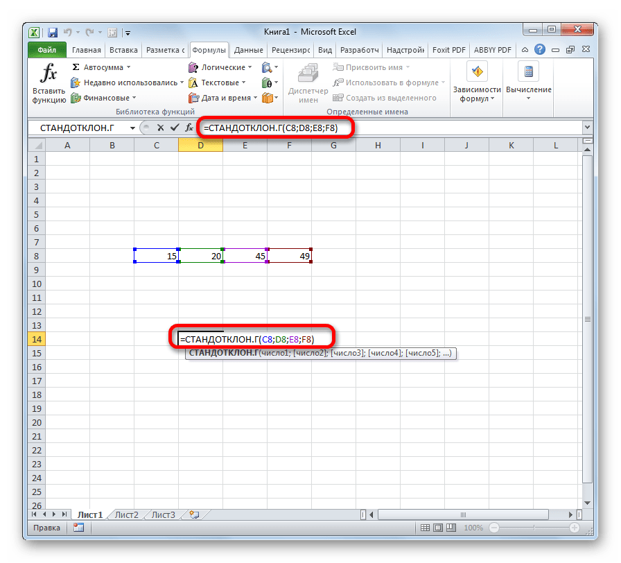

As you can see, the mechanism for calculating standard deviation in Excel is very simple. The user only needs to enter numbers from the population or references to the cells that contain them. All calculations are performed by the program itself. It is much more difficult to understand what the calculated indicator is and how the calculation results can be applied in practice. But understanding this already relates more to the field of statistics than to learning to work with software.