Consider the Normal distribution. Using the functionMS EXCELNORM.DIST() Let's plot the distribution function and probability density. We will generate an array of random numbers distributed according to the normal law, and evaluate the distribution parameters, mean value and standard deviation.
Normal distribution(also called Gaussian distribution) is the most important in both theory and quality control system applications. Importance of value Normal distribution(English) Normaldistribution) in many areas of science follows from probability theory.
Definition: Random value x distributed across normal law if it has:
Normal distribution depends on two parameters: μ (mu)- is , and σ ( sigma)- is (standard deviation). The parameter μ determines the position of the center probability density normal distribution, and σ is the spread relative to the center (average).
Note: The influence of parameters μ and σ on the shape of the distribution is described in the article about, and in example file on the Influence of parameters sheet You can use it to observe the change in the shape of the curve.

Normal distribution in MS EXCEL
In MS EXCEL, starting from version 2010, for Normal distribution there is a function NORM.DIST(), the English name is NORM.DIST(), which allows you to calculate probability density(see formula above) and cumulative distribution function(the probability that a random variable X distributed over normal law, will take a value less than or equal to x). Calculations in the latter case are made using the following formula:

The above distribution is designated N(μ; σ). The notation via N(μ; σ 2).
Note: Before MS EXCEL 2010, EXCEL only had the NORMDIST() function, which also allows you to calculate the distribution function and probability density. NORMDIST() is left in MS EXCEL 2010 for compatibility.
Standard normal distribution
Standard normal distribution called normal distribution with μ=0 and σ=1. The above distribution is designated N(0;1).
Note: In the literature for a random variable distributed over standard normal law a special designation z is assigned.
Any normal distribution can be converted to standard via variable replacement z=(x-μ)/σ . This conversion process is called standardization.
Note: MS EXCEL has a NORMALIZE() function that performs the above conversion. Although in MS EXCEL this transformation is called for some reason normalization. Formulas =(x-μ)/σ and =NORMALIZATION(x;μ;σ) will return the same result.
In MS EXCEL 2010 for There is a special function NORM.ST.DIST() and its legacy variant NORMSDIST() that performs similar calculations.
We will demonstrate how the standardization process is carried out in MS EXCEL normal distribution N(1,5; 2).
To do this, we calculate the probability that a random variable distributed over normal law N(1.5; 2), less than or equal to 2.5. The formula looks like this: =NORMAL.DIST(2.5, 1.5, 2, TRUE)=0.691462. By making a variable change z=(2,5-1,5)/2=0,5 , write down the formula for calculating Standard normal distribution:=NORM.ST.DIST(0.5, TRUE)=0,691462.
Naturally, both formulas give the same results (see. example sheet file Example).
note that standardization only applies to (argument integral equals TRUE), and not to probability density.
Note: In the literature for a function that calculates the probabilities of a random variable distributed over standard normal law a special designation Ф(z) is fixed. In MS EXCEL this function is calculated using the formula
=NORM.ST.DIST(z;TRUE). Calculations are made using the formula

Due to the parity of the function distribution f(x), namely f(x)=f(-x), function standard normal distribution has the property Ф(-x)=1-Ф(x).
Inverse functions
Function NORM.ST.DIST(x;TRUE) calculates the probability P that a random variable X will take a value less than or equal to x. But often the reverse calculation is required: knowing the probability P, you need to calculate the value of x. The calculated value of x is called standard normal distribution.
In MS EXCEL for calculation quantiles use the NORM.ST.INV() and NORM.INV() functions.
Function graphs
The example file contains distribution density graphs probabilities and cumulative distribution function.

As is known, about 68% of the values selected from the population having normal distribution, are within 1 standard deviation (σ) of μ (mean or mathematical expectation); about 95% are within 2 σ, and already 99% of the values are within 3 σ. Make sure of this for standard normal distribution you can write the formula:
=NORM.ST.DIST(1,TRUE)-NORM.ST.DIST(-1,TRUE)
which will return a value of 68.2689% - this is the percentage of values that are within +/-1 standard deviation of average(cm. Graph sheet in example file).
Due to the parity of the function density standard normal distributions: f(x)= f(-X), function standard normal distribution has the property F(-x)=1-F(x). Therefore, the above formula can be simplified:
=2*NORM.ST.DIST(1;TRUE)-1
For free normal distribution functions N(μ; σ) similar calculations should be made using the formula:
2* NORM.DIST(μ+1*σ;μ;σ;TRUE)-1
The above probability calculations are required for .
Note: For ease of writing, formulas in the example file are created for the distribution parameters: μ and σ.
Random number generation
Let's generate 3 arrays of 100 numbers each with different μ and σ. To do this in the window Generation random numbers set the following values for each pair of parameters:

Note: If you set the option Random scattering (Random Seed), then you can select a specific random set of generated numbers. For example, by setting this option to 25, you can generate the same sets of random numbers on different computers (if, of course, other distribution parameters are the same). The option value can take integer values from 1 to 32,767. Option name Random scattering may be confusing. It would be better to translate it as Dial number with random numbers.
As a result, we will have 3 columns of numbers, based on which we can estimate the parameters of the distribution from which the sample was taken: μ and σ . An estimate for μ can be done using the AVERAGE() function, and for σ using the STANDARDEV.B() function, see example file sheet Generation.
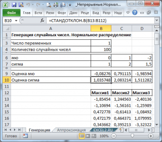
Note: To generate an array of numbers distributed over normal law, you can use the formula =NORM.INV(RAND(),μ,σ). The RAND() function generates from 0 to 1, which exactly corresponds to the range of probability changes (see. example file sheet Generation).
Tasks
Problem 1. The company produces nylon threads with an average strength of 41 MPa and a standard deviation of 2 MPa. The consumer wants to purchase threads with a strength of at least 36 MPa. Calculate the probability that batches of filament produced by a company for a customer will meet or exceed specifications.
Solution1: =1-NORM.DIST(36,41,2,TRUE)
Problem 2. The company produces pipes with an average outer diameter of 20.20 mm and a standard deviation of 0.25 mm. According to the technical specifications, pipes are considered suitable if the diameter is within 20.00 +/- 0.40 mm. What proportion of manufactured pipes comply with specifications?
Solution2: = NORM.DIST(20.00+0.40;20.20;0.25;TRUE)- NORM.DIST(20.00-0.40;20.20;0.25)
In the figure below, the range of diameter values that meets the specification requirements is highlighted.

The solution is given in example file task sheet.
Problem 3. The company produces pipes with an average outer diameter of 20.20 mm and a standard deviation of 0.25 mm. The outer diameter must not exceed a certain value (assuming the lower limit is not important). What upper limit in the technical specifications must be set so that 97.5% of all manufactured products meet it?
Solution3: =NORM.OBR(0.975; 20.20; 0.25)=20.6899 or
=NORM.ST.REV(0.975)*0.25+20.2("destandardization" was carried out, see above)
Problem 4. Finding parameters normal distribution according to the values of 2 (or ).
Suppose it is known that the random variable has a normal distribution, but its parameters are not known, but only the 2nd percentile(for example 0.5- percentile, i.e. median and 0.95th percentile). Because is known, then we know, i.e. μ. To find you need to use .
The solution is given in example file task sheet.
Note: Before MS EXCEL 2010, EXCEL had the NORMINV() and NORMSINV() functions, which are equivalent to NORM.INV() and NORM.ST.INV() . NORMBR() and NORMSINV() are left in MS EXCEL 2010 and higher only for compatibility.
Linear combinations of normally distributed random variables
It is known that a linear combination of normally distributed random variables x(i) with parameters μ (i) and σ (i) is also normally distributed. For example, if the random variable Y=x(1)+x(2), then Y will have a distribution with parameters μ (1)+ μ(2) And ROOT(σ(1)^2+ σ(2)^2). Let's verify this using MS EXCEL.
Brief theory
Normal is the probability distribution of a continuous random variable whose density has the form:
where is the mathematical expectation and is the standard deviation.
Probability that it will take a value belonging to the interval:
where is the Laplace function:
The probability that the absolute value of the deviation is less than a positive number:
In particular, when the equality holds:
When solving problems that practice poses, one has to deal with various distributions of continuous random variables.
In addition to the normal distribution, the basic laws of distribution of continuous random variables:
Example of problem solution
A part is made on a machine. Its length is a random variable distributed according to a normal law with parameters , . Find the probability that the length of the part will be between 22 and 24.2 cm. What deviation of the length of the part from can be guaranteed with a probability of 0.92; 0.98? Within what limits, symmetrical with respect to , will almost all dimensions of the parts lie?
Solution:
The probability that a random variable distributed according to a normal law will be in the interval:
We get:
The probability that a normally distributed random variable will deviate from the mean by no more than .
The law of normal probability distribution of a continuous random variable occupies a special place among various theoretical laws, since it is fundamental in many practical studies. It describes most random phenomena associated with production processes.
Random phenomena that obey the normal distribution law include measurement errors of production parameters, the distribution of technological manufacturing errors, the height and weight of most biological objects, etc.
Normal is the law of probability distribution of a continuous random variable, which is described by a differential function
a - mathematical expectation of a random variable;
Standard deviation of a normal distribution.
The graph of the differential function of the normal distribution is called a normal curve (Gaussian curve) (Fig. 7).

Rice. 7 Gaussian curve
Properties of a normal curve (Gaussian curve):
1. the curve is symmetrical about the straight line x = a;
2. the normal curve is located above the X axis, i.e., for all values of X, the function f(x) is always positive;
3. The ox axis is the horizontal asymptote of the graph, because
4. for x = a, the function f(x) has a maximum equal to
![]() ,
,
at points A and B at and the curve has inflection points whose ordinates are equal.
![]()
At the same time, the probability that the absolute value of the deviation of a normally distributed random variable from its mathematical expectation will not exceed the standard deviation is equal to 0.6826.
at points E and G, for and , the value of the function f(x) is equal to
![]()
and the probability that the absolute value of the deviation of a normally distributed random variable from its mathematical expectation will not exceed twice the standard deviation is 0.9544.
Asymptotically approaching the x-axis, the Gaussian curve at points C and D, at and , approaches the x-axis very close. At these points the value of the function f(x) is very small
![]()
and the probability that the absolute value of the deviation of a normally distributed random variable from its mathematical expectation will not exceed three times the standard deviation is 0.9973. This property of the Gaussian curve is called " three sigma rule".
If a random variable is distributed normally, then the absolute value of its deviation from the mathematical expectation does not exceed three times the standard deviation.
Changing the value of the parameter a (the mathematical expectation of a random variable) does not change the shape of the normal curve, but only leads to its displacement along the X axis: to the right if a increases, and to the left if a decreases.
When a=0, the normal curve is symmetrical about the ordinate.
Changing the value of the parameter (standard deviation) changes the shape of the normal curve: with increasing ordinates of the normal curve they decrease, the curve stretches along the X axis and is pressed against it. As it decreases, the ordinates of the normal curve increase, the curve shrinks along the X axis and becomes more “pointy.”
At the same time, for any values and the area bounded by the normal curve and the X axis remains equal to one (i.e., the probability that a normally distributed random variable will take a value bounded on the X axis of the normal curve is equal to 1).
Normal distribution with arbitrary parameters and , i.e., described by a differential function

called general normal distribution.
The normal distribution with parameters is called normalized distribution(Fig. 8). In a normalized distribution, the differential distribution function is equal to:

Rice. 8 Normalized curve
The cumulative function of the general normal distribution has the form:
Let the random variable X be distributed according to the normal law in the interval (c, d). Then the probability that X will take a value belonging to the interval (c, d) is equal to
![]()
Example. The random variable X is distributed according to the normal law. The mathematical expectation and standard deviation of this random variable are equal to a=30 and . Find the probability that X will take a value in the interval (10, 50).
By condition: . Then
Using ready-made Laplace tables (see Appendix 3), we have.
(real, strictly positive)
Normal distribution, also called Gaussian distribution or Gauss - Laplace- probability distribution, which in the one-dimensional case is specified by the probability density function coinciding with the Gaussian function:
f (x) = 1 σ 2 π e − (x − μ) 2 2 σ 2 , (\displaystyle f(x)=(\frac (1)(\sigma (\sqrt (2\pi ))))\ ;e^(-(\frac ((x-\mu)^(2))(2\sigma ^(2)))),)where the parameter μ is the expectation (mean value), median and mode of the distribution, and the parameter σ is the standard deviation (σ² is the dispersion) of the distribution.
Thus, the one-dimensional normal distribution is a two-parameter family of distributions. The multivariate case is described in the article “Multivariate normal distribution”.
Standard normal distribution is called a normal distribution with mathematical expectation μ = 0 and standard deviation σ = 1.
Encyclopedic YouTube
-
1 / 5
The importance of the normal distribution in many fields of science (for example, mathematical statistics and statistical physics) follows from the central limit theorem of probability theory. If the result of an observation is the sum of many random weakly interdependent quantities, each of which makes a small contribution relative to the total sum, then as the number of terms increases, the distribution of the centered and normalized result tends to be normal. This law of probability theory results in the widespread distribution of the normal distribution, which was one of the reasons for its name.
Properties
Moments
If random variables X 1 (\displaystyle X_(1)) And X 2 (\displaystyle X_(2)) are independent and have a normal distribution with mathematical expectations μ 1 (\displaystyle \mu _(1)) And μ 2 (\displaystyle \mu _(2)) and variances σ 1 2 (\displaystyle \sigma _(1)^(2)) And σ 2 2 (\displaystyle \sigma _(2)^(2)) accordingly, then X 1 + X 2 (\displaystyle X_(1)+X_(2)) also has a normal distribution with mathematical expectation μ 1 + μ 2 (\displaystyle \mu _(1)+\mu _(2)) and variance σ 1 2 + σ 2 2 . (\displaystyle \sigma _(1)^(2)+\sigma _(2)^(2).) It follows that a normal random variable can be represented as the sum of an arbitrary number of independent normal random variables.
Maximum entropy
The normal distribution has the maximum differential entropy among all continuous distributions whose variance does not exceed a given value.
Modeling normal pseudorandom variables
The simplest approximate modeling methods are based on the central limit theorem. Namely, if you add several independent identically distributed quantities with finite variance, then the sum will be distributed approximately Fine. For example, if you add 100 independent ones as standard evenly distributed random variables, then the distribution of the sum will be approximately normal.
For programmatic generation of normally distributed pseudorandom variables, it is preferable to use the Box-Muller transformation. It allows you to generate one normally distributed value based on one uniformly distributed value.
Normal distribution in nature and applications
Normal distribution is often found in nature. For example, the following random variables are well modeled by the normal distribution:
- deviation when shooting.
- measurement errors (however, the errors of some measuring instruments do not have normal distributions).
- some characteristics of living organisms in a population.
This distribution is so widespread because it is an infinitely divisible continuous distribution with finite variance. Therefore, some others approach it in the limit, for example, binomial and Poisson. This distribution models many non-deterministic physical processes.
Relationship with other distributions
- The normal distribution is a Pearson type XI distribution.
- The ratio of a pair of independent standard normally distributed random variables has a Cauchy distribution. That is, if the random variable X (\displaystyle X) represents the relation X = Y / Z (\displaystyle X=Y/Z)(Where Y (\displaystyle Y) And Z (\displaystyle Z)- independent standard normal random variables), then it will have a Cauchy distribution.
- If z 1 , … , z k (\displaystyle z_(1),\ldots ,z_(k))- jointly independent standard normal random variables, that is z i ∼ N (0 , 1) (\displaystyle z_(i)\sim N\left(0,1\right)), then the random variable x = z 1 2 + … + z k 2 (\displaystyle x=z_(1)^(2)+\ldots +z_(k)^(2)) has a chi-square distribution with k degrees of freedom.
- If the random variable X (\displaystyle X) is subject to lognormal distribution, then its natural logarithm has a normal distribution. That is, if X ∼ L o g N (μ , σ 2) (\displaystyle X\sim \mathrm (LogN) \left(\mu ,\sigma ^(2)\right)), That Y = ln (X) ∼ N (μ , σ 2) (\displaystyle Y=\ln \left(X\right)\sim \mathrm (N) \left(\mu ,\sigma ^(2)\right )). And vice versa, if Y ∼ N (μ , σ 2) (\displaystyle Y\sim \mathrm (N) \left(\mu ,\sigma ^(2)\right)), That X = exp (Y) ∼ L o g N (μ , σ 2) (\displaystyle X=\exp \left(Y\right)\sim \mathrm (LogN) \left(\mu ,\sigma ^(2) \right)).
- The ratio of the squares of two standard normal random variables has
Random if, as a result of experiment, it can take on real values with certain probabilities. The most complete, comprehensive characteristic of a random variable is the distribution law. The distribution law is a function (table, graph, formula) that allows you to determine the probability that a random variable X takes a certain value xi or falls into a certain interval. If a random variable has a given distribution law, then it is said that it is distributed according to this law or obeys this distribution law.
Every distribution law is a function that completely describes a random variable from a probabilistic point of view. In practice, the probability distribution of a random variable X often has to be judged only from test results.
Normal distribution
Normal distribution, also called the Gaussian distribution, is a probability distribution that plays a critical role in many fields of knowledge, especially in physics. A physical quantity follows a normal distribution when it is subject to the influence of a huge number of random noises. It is clear that this situation is extremely common, so we can say that of all the distributions, the normal distribution is the most common in nature - hence one of its names.
The normal distribution depends on two parameters - displacement and scale, that is, from a mathematical point of view, it is not one distribution, but a whole family of them. The parameter values correspond to the values of the mean (mathematical expectation) and spread (standard deviation).


The standard normal distribution is a normal distribution with a mathematical expectation of 0 and a standard deviation of 1.


Asymmetry coefficient

The skewness coefficient is positive if the right tail of the distribution is longer than the left, and negative otherwise.
If the distribution is symmetrical relative to the mathematical expectation, then its asymmetry coefficient is zero.

The sample skewness coefficient is used to test the distribution for symmetry as well as a rough preliminary test for normality. It allows you to reject, but does not allow you to accept, the normality hypothesis.
Kurtosis coefficient

The kurtosis coefficient (peakness coefficient) is a measure of the sharpness of the peak of the distribution of a random variable.
“Minus three” at the end of the formula is introduced so that the kurtosis coefficient of the normal distribution is equal to zero. It is positive if the peak of the distribution around the mathematical expectation is sharp, and negative if the peak is smooth.

Moments of a random variable
The moment of a random variable is a numerical characteristic of the distribution of a given random variable.